Logic Lessons: Hypothesis Testing

Lesson 4

I know this will make me sound like a nerd, but hypothesis testing is one of my favorite parts of data analysis/statistics! Not only is it a key part of the scientific method, but it’s frequently used to determine the validity of a mathematical relationship. Hypothesis testing between variables helps determine if their relationship is statistically significant, but what is it and how is it done?

What is a hypothesis?

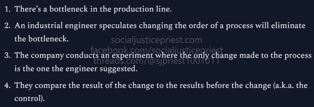
A hypothesis is an educated guess. The scientific method starts with a question. A hypothesis is logical answer to that question. To reuse the Lean Six Sigma example from the previous article (also reposted above), the question would be, “Why is there a bottleneck in the production line?” The hypothesis is the industrial engineer saying, “I think the order we process the widgets is causing the bottleneck.”

How is hypothesis testing done?

It depends on the goal and the type of available data. Is the data from a randomized, controlled experiment (like the kind from the Lean Six Sigma Example) or is it observational data (like my advanced economies data)?

Some steps are the same for both types of data. All hypothesis testing follows the same pattern. The tester forms two hypotheses: the null hypothesis (H₀) and the alternate hypothesis (H_A). The H₀ is the “default” hypothesis. It states the change the tester made or the relationship they observed is not statistically significant. H_A is the opposite, the change made or relationship observed is statistically significant. The goal of a hypothesis test is not to “prove” H_A, but to show we can confidently reject H₀ because our gathered data is unlikely (low p-value) to happen by chance. Since inductive reasoning doesn’t deal in proofs, it’s impossible to “accept” the H_A. Because hypothesis testing can’t prove H_A, it’s subject to errors.

There are two types of errors: type 1 errors and type 2 errors. A type 1 error is a false positive. In other words, the tester wrongfully rejects the null hypothesis. A type 2 error is a false negative. The tester maintains the null hypothesis when they should’ve rejected it. These mistakes can happen when there are errors in the experiment, like an insufficient sample size, for example. While z-testing is good for experiments with thirty samples or more, smaller samples require t-testing. T-testing is the most common form of hypothesis testing. It’s similar to z-testing, but accounts for the extra noise associated with small sample sizes. If the testers accidentally used z-testing instead of t-testing, they could reach an erroneous conclusion.

With experimental data, the tester has complete control over the environment. Because they can control for outside variables, a significant p-value directly hints at a causal link. A/B Testing is a common form of gathering experimental data. A company tests two versions (A & B) of a website or advertisement in a randomized controlled experiment. Usually, A is the original version of the website and B is a version with a change. The company tests a new website feature on a random group of users. If the test yields a low p-value, they know the feature caused the change (good or bad) in user behavior.

The gold standard for experimental data is a p-value of 0.05, meaning there’s a less than 5% chance the results of the experiment were statistical noise.

Observational data is more complicated. As the name suggests, observational data is data acquired through observing events in nature, also known as observational studies or natural experiments. While hypothesis testing here is still important, it can’t be used to establish causation. What it can do is show an observed relationship between the independent and dependent variables is not due to statistical noise/random chance. While this doesn’t show the independent variable causes the dependent one, it shows a relationship definitely exists.

Because observational data is often limited (e.g. the number of countries with advanced economies is currently thirty-seven), it’s difficult to achieve a lower p-value without a strong relationship (a high r² in regression analysis). Small samples make it harder to achieve statistical significance because the data is “noisier.” I will be using a 90% confidence level (p-value = 0.10 or lower) for my “What Does the Data Say?” series to account for this. While this means my hypothesis tests will have a lower, more lenient threshold for significance, it will allow me to avoid more type 2 errors with such a small sample size.

I’m concerned about avoiding type 2 errors because the main purpose of the “What Does the Data Say?” series is to look at the relationships between multiple economic metrics that describe the prosperity and quality-of-life among the advanced economies. Since one of the themes of the series is pointing out the lack of causality between two metrics by finding no correlation, I want to make sure I’m not writing off any potential relationships just to get a “win.”

After choosing a confidence level, the important part is sticking with it. This is where many people make mistakes. Humans are biased toward beliefs they want to be true. This causes people to move the goalpost after the testing is done so their hypotheses support what they already believe. Going back to the Lean Six Sigma example, if the industrial engineer really wanted their hypothesis to be correct, they might be tempted to accept a calculated p-value of 0.07 because it’s “close enough.” While this may make the engineer feel good, it does the company a disservice by adding type I errors (false positives) to their improvement process.

So why bother?

To bring this back to my “What Does the Data Say?” series, hypothesis testing allows me to determine if there’s statistically significant evidence of a relationship between two variables. In the case of linear relationships, like the ones I deal with in my data sets, the establishment of a relationship sets the stage for further experimentation and/or observation. Indeed, multiple economists have won Nobel prizes by doing exactly this. Dr. David Card “proved” using observational data that immigrants don’t depress wages (Magesan, 2021). Another example is the economists, Dr. David Card (again), Dr. Joshua Angrist, and Dr. Guido Imbens, who “proved” minimum wage increases don’t cost jobs by observing natural experiments between multiple sets of towns where the main difference was one state having a higher minimum wage than the other (Nobel Prize Outreach 2026, 2026). Again, “proved” is in quotes because what they actually did was achieve statistical significance, which is as close to definitive proof as empirical analysis allows. All three won the 2021 Nobel Prize for their work.

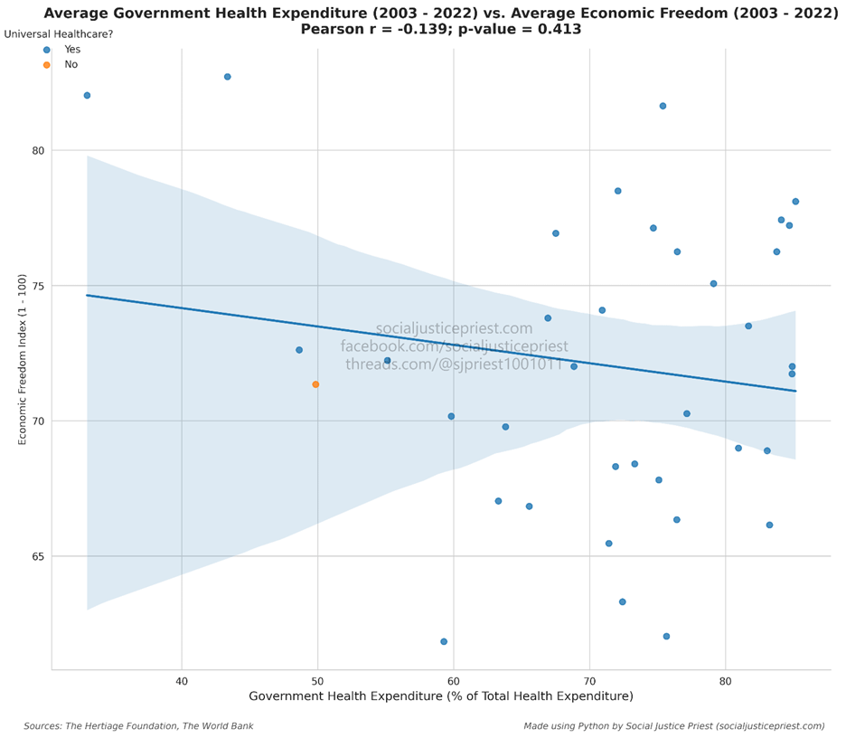
Conversely, hypothesis testing allows me to determine there is no statistically significant evidence of a relationship between two variables, and this is where it gets fun. I used hypothesis testing in the above chart to determine there was no statistically significant evidence of a relationship between government spending on healthcare (as a percentage of all healthcare expenditure) and the Economic Freedom Index. This means politicians claiming the increased government expenditure associated with universal healthcare would destroy economic freedom have no evidence to back up their claims!

Sources:

Magesan, A. (2021, October 26). Nobel Winner David Card Shows Immigrants Don’t Reduce the Wages of Native-Born Workers. University of Calgary. https://ucalgary.ca/news/nobel-winner-david-card-shows-immigrants-dont-reduce-wages-native-born-workers

Munro, R. A., Ramu, G., & Zrymiak, D. J. (2022). ASQ Certified Six Sigma Green Belt Handbook (3rd Edition). American Society for Quality.

Nobel Prize Outreach 2026. (2026). The Sveriges Riksbank Prize in Economic Sciences in Memory of Alfred Nobel 2021. NobelPrize.org. https://www.nobelprize.org/prizes/economic-sciences/2021/summary/

Wheelan, C. J. (2014). Naked Statistics: Stripping the Dread from the Data. W.W. Norton & Company.

Enjoying my content?